Fwd/Inv Kinematics

Introduction

Kinematics here is distinct from Newton's kinematic equations. Rather than describing the motion of an object or particle, we're discussing the motion of connected bodies to calculate a final position and orientation. This is known as Forward or Direct Kinematics.

As the name would imply, there's also something called Backwards or Inverse Kinematics. This is a much harder problem of finding a viable set of orientations of connected parts that can achieve a desired final configuration.

Forward Kinematics

Forward kinematics is a process of manipulating bodies (frequently described as vectors) to calculate a new location and orientation.

In one of our math articles, we explain how vectors can be added and subtracted. When calculating forward kinematics, it's important to understand how to define the vectors. The base vector should be defined with respect to an anchoring point, and the length of the vector should be from the attachment point (frequently this is the center of an axle) up to another attachment point or axle center.

Here you can see a robot arranged at right angles, where +x is to the right, and +y is up.
v1 = [0,d1]
v2 = [0,d2]
v3 = [de,0]

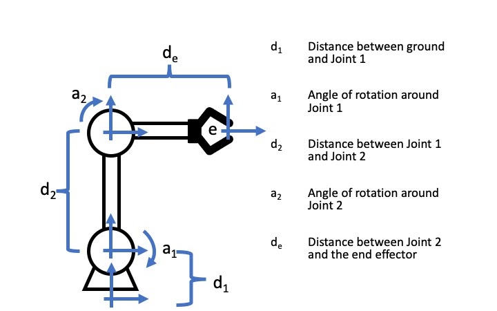
Notice that the length of v1, v2, and v3 are defined by the the distance from the anchor point to an axle, axle to axle, or axle to "end effector". Also keep in mind that the vectors we described are the current orientation. Each body has a base ordefault decription, and an effective description. This is because as we scale up from 1 dimension to 2-3 dimenions we start to factor in rotation.

Rotation doesn't change the length of the vector, it only changes the values that make it up. Think back to our unit circle. That is a vector of length 1, and as you rotate the vector around you get different values. The Trig there works well when the vector is simply [1, 0], however we usually don't have that luxery in the real world. We have to use something called a rotation matrix to change from the base values, to the effective values.

With this matrix and your rotation angle set to 0 degrees, this forms something called the identity matrix. Which is a fancy phrase that basically means "multiply by 1", or do nothing.

In 3 dimensions you might see the matrices look a little different. These are something called Euler Angle rotations.

If you know your linear algebra from class, you might recognize that the last matrix in the list is the same as the 2 by 2 matrix for points in 3d space. In other words, you could use the same x and y points, and an arbitrary point in the z dimension, and using that last matrix will transform the points in the same way as the 2 by 2 matrix.

When we combine both of these together we can get more sophisticated conversions from one coordinate from to another.

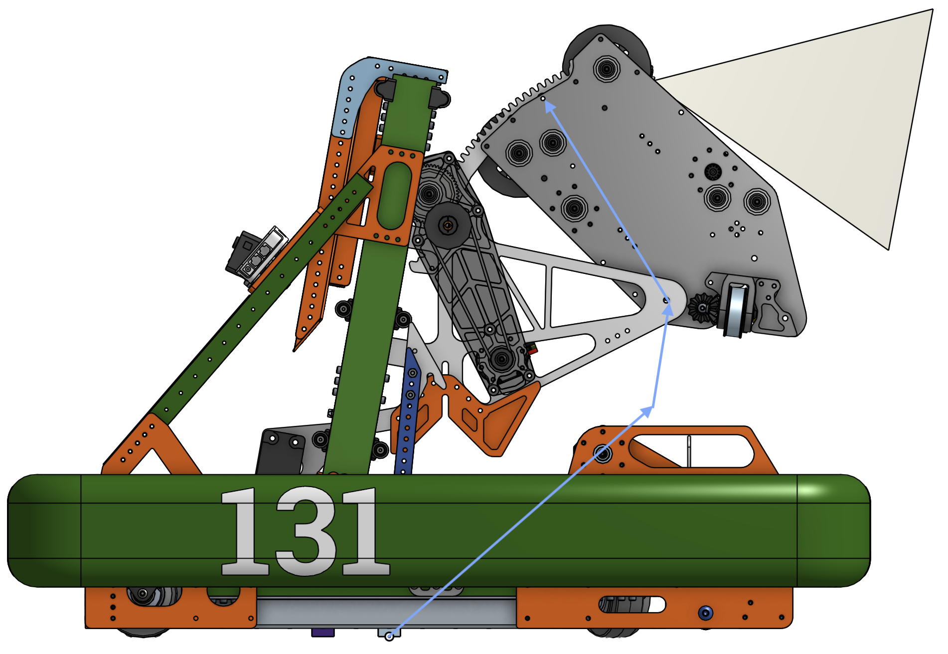
This is Double Time, the robot from 2024's game Crescendo. Notice how our vectors are not neatly aligned along an axis, also keep in mind that the axis are +x left, +z up. We don't use y's because +y is the left side of the robot, which is where the camera is located. From our source code, the 3 vectors are
V1 = [-0.299, 0, 0.277], V2 = [-0.082, 0, 0.425], V3 = [0.18, 0, 0.177].

Each of the vectors does something important. The first one is a constant vector, it calculates a joint behind the robot based on the current position and orientation of the robot. The next vector is the lift vector, which is normalized to a unit vector, and that is then multiplied by the height of the lift along its track. The third vector must be rotated around its axle, as it indicates where the release point of the launcher with respect to that axle. That uses the R_y rotation matrix.

This gives us a robot relative vector that describes the game piece release point relative to the robot origin. To make that a field relative vector, the resulting vector must be rotated again based on the robot's field pose. In most cases, that means you just do one more rotation, yielding our final 3d point on the field
[x'', y'', z'']. Note that because this is now robot relative, and the robot is presumably flat on the ground, we only multiply by R_z. Other rare robot pose orientations would have different rotations used.

Inverse Kinematics

This is a section on inverse kinematics. Deducing orientations of segments to achieve a desired end location and orientation.

The thing that makes inverse kinematics difficult is the potentially infinite set of configurations. You can't pick an angle or motor position, when there are 360 degrees of viable data point. You could pick a random value in a range, but aligning that point with other joints in the system leads to cascading constraints that may have to be undone and recalculated.

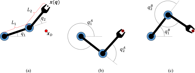
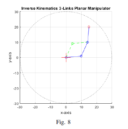
Lets look at a really basic situation. In the above image, you can see the state of the arm, and the red dot is where the arm wants to end at. In this trivial example, there are two ways to get there! Image B and C show the two solutions. By adding another joint, the number of solutions hits an infinite number of solutions.

We can't really resolve this cleanly. There are many techniques for resolving inverse kinematic problems; Jacobian, Gradiant Descent, and Heuristic to name a few. In the example below, you can see two solutions because the technique used applied a specific constraint, that the last segment would approach from a specific angle/position. This is called the heuristic model. Gradiant descent involves slightly changing some or many of the angles to achieve the new target. We will not be addressing Jacobian solutions in this article, but encourage our daring readers to check it out themselves.

Somewhat paradoxically, introducing constraints can make many problems in life easier. Formal proofs in math benefit from this in Proof by Cases, it can encourage creative thinking in difficult environments, and eliminating options can help people with Analysis Paralysis.

As a result, most complex systems function with these simpler faster models, and typically don't use a Jacobian model, and they eliminate as many joints from the system as they can afford. This also benefits the mechanical team, as joints are some of the weaker parts of a robot.

• Robotic Systems, Duke.
• Forward and Reverse Kinematics for 3R Planar Manipulator

2025 Kinematics Model

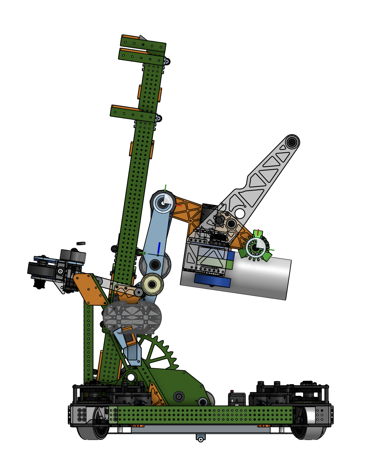
So lets take a look at how some of these concepts can be used, and look at the 2 jointed robot design from 2025, Angler.

There are many ligaments that make up this robot. When you trace the side profile of the robot, you can group these lines into several groups. See the image on the right for each line segment, and note the joints indicated by the red dots. Also, each group has the same color for all line segments. What you can gather from this is that each group can be simplified.

You can simplify by looking at the group, and identifying the segments with a locked or fixed angle between them. This typically means the two segments can be added together. This is best done with vectors. If you add all of the vectors within a group together, this should bring you to the next joint, or linear component.

The interactive demo below shows the simplified kinematic model, note how the parts all move circularly around their corresponding joints.

Once we have our simplified kinematic model, we can leverage that with inverse kinematics. Lets break down each ligament, the local coordinate frame of each, and how to derive unknown angles and lengths given a target end effector state.

The first step is to start at the origin, and trace the vectors forward as much as possible. In our 2025 robot, this first ligament is a constant offset from the robot origin to a joint, and we need to know what the effective origin is for the inverse calculations. So we make a note of where this axle is, and move to the opposite side of the problem.

Just like we looked at the initial ligament, we're going to do the same thing with the final ligament that connects to the end effector. One of the requirements of end effectors with inverse kinematics is that you need to know both their position and theirorientation. Knowing this, and the length of the final ligament, we can calculate where the nearest joint lands.

Thankfully, the 2025 robot is simple enough that we don't have any more joints! We only have a linear slide (elevator, lift, what have you), and a ligament at a fixed angle representing the carriage mount.

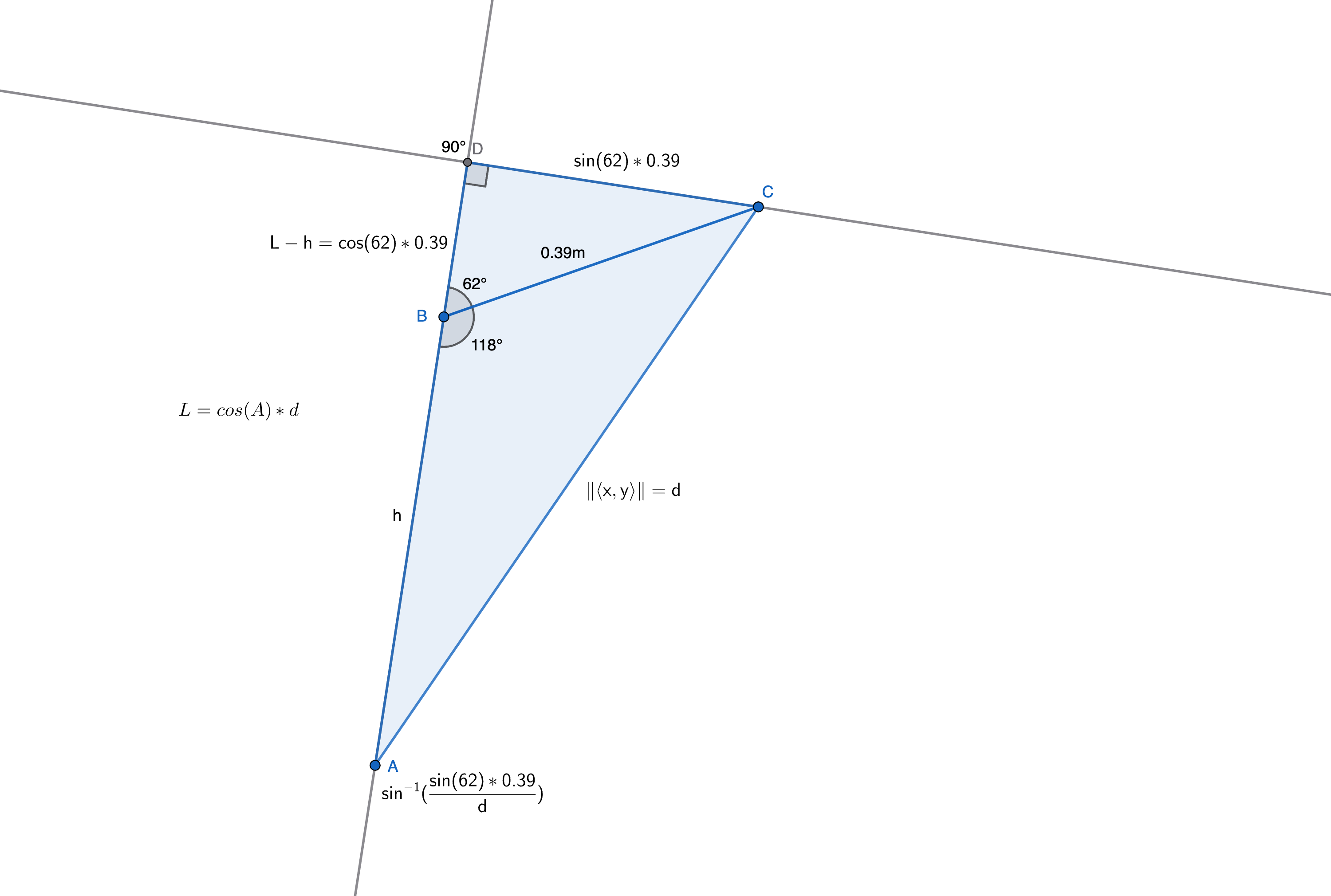
This means we have 2 points in space, with several knowns and unknowns. We can leverage our trigonometry skills to calculate the angle of our lift, the length of it, and the relative angle of our end effector all relatively easily!

As we set up our triangle, it's important to annotate what we know, and what we want to know. We know the vector of our problem space, it's the gap between our joints and it's indicated by the <x, y> along one edge. We also know the length of the carriage attachment, marked as 0.39 (meters). Lastly, we know the angle of the carriage mounting relative to the direction of the lift, marked as 118 degrees.

Now notice that we have not just one triangle here, but 2. That's because this problem is easier to solve by forming a right hand triangle out of the existing known data. We can derive the lengths of all 3 sides because of our skills in Trig! Why might this be useful? because it allows us to combine the two triangles into a larger right triangle, and solve the lower angle this way, and ultimately find the length h. This length h is the length of our lift!